
Every business experiment has a price. The decisive question is whether the company pays for it inside a model or directly in the market.
Imagine two companies facing the same problem. A major customer has delayed payment. Demand is weakening, input costs are rising and both companies must decide whether to borrow, accelerate collections, reduce inventory, postpone investment or adjust prices.
The first company integrates its operational and financial evidence, evaluates thousands of possible cash-flow paths, identifies its binding constraints, compares available interventions and measures the downside risk of each decision.
The second reconstructs its position manually, changes several assumptions in a spreadsheet, discusses the available options and selects the one that appears most reasonable. Its management may be experienced and its judgement may be sound. But the real cost of the decision will only become visible after it has been implemented.
Both businesses have ideas. Both possess data. Both can prepare forecasts. But they do not face the same cost of learning.
The first company experiments inside its model. The second is forced to experiment inside the business.
That difference is becoming one of the most important structural divisions in modern competition.
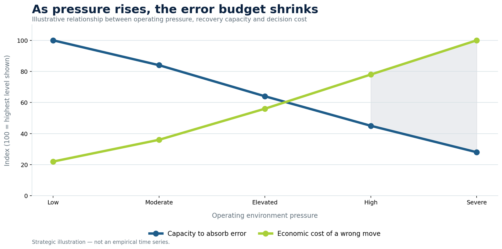
The disappearing margin for error
Trial and error has always been part of business. A company changes a price, increases inventory, employs more people, enters a new market or invests in new technology and then observes what happens.
That process was never free. However, businesses operating with stronger margins, cheaper financing, slower technological renewal and more forgiving supply structures had greater capacity to absorb an imperfect decision.
That capacity is narrowing.
Late payments are estimated to cost the UK economy almost £11 billion annually. Approximately 1.5 million businesses are affected each year, while an estimated £26 billion is owed in late payments at any given time. The same research estimated that 14,000 businesses close each year because of late payment.1
Company insolvency volumes rose above pre-pandemic levels after 2021, with 2023 producing a 30-year high. The position subsequently improved, but one in 196 companies on the effective register still entered insolvency in the twelve months to May 2026.2
The issue is not that every business faces immediate collapse. It is that the economic space available for absorbing repeated mistakes is becoming smaller.
A pricing error damages contribution. A purchasing error traps cash in inventory. A poorly timed investment increases financing pressure. A delayed operational response turns a manageable cash trough into a liquidity event. At the same time, companies must renew technology faster if they want to preserve productivity and reduce dependency.
Every business therefore operates with an effective error budget:
where is available liquidity, unused capacity, margin headroom, financing access and current risk exposure.
As this budget contracts, optimisation moves from an analytical enhancement to a methodological necessity.
A forecast is not a decision
Reporting describes what has happened. Forecasting estimates what is likely to happen. Neither automatically determines the best response.
If a 13-week forecast shows cash falling below the required safety reserve in week eight, it has identified the condition. It has not decided whether management should borrow, accelerate selected receivables, renegotiate supplier timing, defer expenditure or combine several interventions.
A forecast shows the trajectory. Optimisation changes it. Learning improves the next intervention.
The complete management cycle is:
This is the direction we are applying in CF Compass: moving from cash visibility through horizon-sensitive forecasting towards risk-adjusted optimisation and continuous recalibration.
But the principle extends far beyond cash. The same structure applies to pricing, inventory, capacity, working capital, investment and resource allocation.
The 13-week cash-flow architecture
A cash-flow model should not treat every week as equally predictable.
In the immediate horizon, the company already knows much of what will happen. Bank balances, issued invoices, payroll, direct debits, approved supplier payments, tax liabilities and committed expenditure provide a relatively firm transactional foundation.
Further into the future, confirmed evidence gives way to expectations. Orders remain uncertain, payment dates become less reliable, costs can change and management must consider several possible business states.
CF Compass therefore separates the forecast horizon into three environments:
| Horizon | Forecasting environment | Primary function |
|---|---|---|
| Weeks 1–4 | Deterministic | Control known and committed cash movements |
| Weeks 4–8 | Hybrid | Combine identifiable evidence with probabilities and sensitivities |
| Weeks 8–13 | Stochastic | Evaluate distributions, regimes and downside risk |
This is not three disconnected forecasts. It is one trajectory that changes its evidential character through time. A possible receipt in week twelve may initially be represented by a distribution. As time progresses, it becomes an expected order, then a confirmed invoice and finally a reconciled bank movement.
The future moves from stochastic possibility towards deterministic evidence.
The model should also understand more than the cash position itself. Let represent cash at time . Cash velocity and acceleration are:
Position shows where the company is. Velocity shows how quickly cash is accumulating or disappearing. Acceleration shows whether that movement is strengthening or weakening.
A company with £500,000 in cash but a weekly velocity of may be in a weaker trajectory than a company with £250,000 and a velocity of .
Cash can still be falling while the decline is decelerating. It can also remain positive while its dynamics are already deteriorating.
A negative result can be improving, while a positive result can already be weakening.
Three models for three management functions
The architecture uses three optimisation models. Their purpose is not to turn management into a mathematics lecture. Each answers a different practical question.
Model 1 — Constrained Position Optimisation
Lagrangian → Newton on the KKT system
This model asks: What is the best feasible combination of actions under the constraints we currently face?
For objective , inequality constraints and equality constraints , the Lagrangian is:
The economically feasible optimum satisfies the KKT conditions:
Newton iteration acts on the resulting nonlinear KKT system :
The model can optimise funding, receipt acceleration, payment timing, expenditure deferral, inventory, capacity and price-volume decisions. Its multipliers also reveal shadow prices: the marginal value of relaxing a cash, credit, capacity or inventory constraint.
Model 2 — Dynamic Trajectory Optimisation
Hamiltonian → Newton shooting with variational equations
This model asks: When should management intervene, and how strongly, to create the best trajectory?
For a state , control and state dynamics , the Hamiltonian is:
The optimal trajectory satisfies:
Cash, inventory and demand change through time. Management interventions therefore have timing, intensity and duration. Borrowing one week too early creates unnecessary interest. Borrowing one week too late may allow a liquidity breach. Discounting inventory too early destroys margin; discounting it too late creates waste.
Newton shooting adjusts the proposed state-costate trajectory towards the required terminal condition. Variational equations show how sensitive the result is to changes in initial conditions and assumptions.
Model 3 — Adaptive Policy Optimisation
Bellman → Newton–Kantorovich policy iteration
This model asks: What should management do next, given the state in which the business actually arrives?
The Bellman equation combines current reward with the expected value of the future state:
Writing the fixed-point problem as , Newton–Kantorovich iteration becomes:
No forecast unfolds exactly as expected. Customers pay late, demand changes, suppliers alter terms and new opportunities appear. Bellman optimisation therefore produces a state-dependent policy rather than one fixed answer.
Lagrange helps management allocate. Hamilton helps management steer. Bellman helps management adapt.
Applied cash-flow optimisation
Consider a company with opening cash of £420,000, a minimum required reserve of £150,000, forecast cash of £62,000 in week eight and a £150,000 revolving credit facility. Customer invoices can be accelerated, selected supplier payments rescheduled and discretionary expenditure deferred.
The forecast identifies an £88,000 breach of the reserve.
One response is to draw £110,000 from the credit facility for five weeks. At an annual interest rate of 9.5% and a 1.5% drawdown fee, the approximate direct cost is:
The action restores the reserve under the central forecast but consumes most of the available facility. If another customer pays late, little emergency headroom remains.
A constrained optimisation model may identify a better combination:
- accelerate £60,000 of selected receivables at a 1% discount;
- reschedule £35,000 of non-critical supplier payments at an estimated economic cost of £350;
- draw £25,000 from the facility;
- protect payroll, critical inventory and essential investment.
The approximate direct cost becomes:
The combination costs approximately £1,102 less and preserves £125,000 of credit capacity.
But the cheapest result under the central forecast is not necessarily optimal. The model must test delayed receipts, customer default, cost shocks, reserve-breach probability, maximum cash drawdown, remaining funding capacity and losses in the worst outcomes.
Conditional Value at Risk makes the tail explicit. For loss and confidence level :
An intervention that saves £1,000 but creates a much larger tail exposure is not optimised. It is merely cheaper under one assumed future.
The objective is to create the strongest viable plan across the range of outcomes the company can realistically face.
Pricing, discounts and perishable inventory
Pricing exposes the danger of optimising one metric in isolation.
Increasing price can improve margin per unit but reduce demand. Reducing price can accelerate sales but destroy contribution. When products are perishable, the model must also consider remaining shelf life, holding cost, waste and the declining opportunity to sell.
A preliminary application we explored used chilled dairy inventory. The model treated inventory as the changing state, price as the control, demand as responsive but uncertain, expiry as a time boundary and waste as an economic penalty.
With inventory and demand , the state evolves as:
The price trajectory can then be framed as:
This remains an application experiment rather than a validated commercial pricing model. A real implementation requires transaction-level evidence, reliable elasticity estimates, seasonality, competitor behaviour, promotion effects, replenishment constraints and out-of-sample testing.
Its value lies in demonstrating the difference between a heuristic and a model.
A heuristic says: Reduce the price by 20% three days before expiry.
The model asks how much inventory remains, how quickly it is selling, how demand responds to price, whether observed elasticity has changed, what waiting costs and which price path produces the strongest risk-adjusted contribution.
The same principle applies to early-payment discounts. A 2% discount on a £100,000 invoice costs £2,000. If it brings payment forward by thirty days while equivalent borrowing costs 9.5% annually, the approximate financing cost is:
Under normal conditions, borrowing may be cheaper than surrendering £2,000 of revenue. But if the credit facility is exhausted, default risk is increasing or the receipt prevents a severe liquidity breach, the discount may still be optimal.
The correct question is not whether the discount accelerates cash. It is whether the economic value and risk reduction created by earlier cash exceed the margin surrendered.
The model must learn with the business
A model is only as good as its data, assumptions and representation of economic reality. But its assumptions do not have to remain static.
A learning optimisation system compares forecast and actual outcomes and updates both its inputs and its future decisions. For parameter vector , a controlled update can be represented as:
The learning rate should reflect sample size, evidence quality, forecast error and structural stability. The system can learn from actual payment delays, customer defaults, demand response, collection interventions, supplier flexibility, cost volatility and movement between favourable, normal and adverse states.
Time therefore performs two opposing functions. Looking forward, it creates uncertainty. Experienced through a learning system, it creates information.
The system must not reinterpret every deviation as a new pattern. That would teach the model to follow noise. Learning requires evidence thresholds, confidence intervals, parameter limits, outlier controls, validation, versioning and the ability to reverse an unstable update.
A heuristic hides its assumptions inside habit. A learning model exposes its assumptions to evidence, measurement and correction.
Optimisation does not create certainty about the outcome. It creates greater confidence that the selected decision is consistent with the available evidence, stated assumptions, constraints and risk limits.
The wall between large companies and SMEs
This is where optimisation becomes a structural economic issue.
The effective cost of one learning iteration can be expressed as:
A large company can automate data preparation, employ specialist teams, run thousands of simulations, discard weak alternatives and distribute the cost across millions of transactions.
An SME may need to collect the data manually, reconstruct the model, purchase external expertise and test the decision directly in its operations. Its cost per shot is higher, while its capacity to absorb failure is lower.
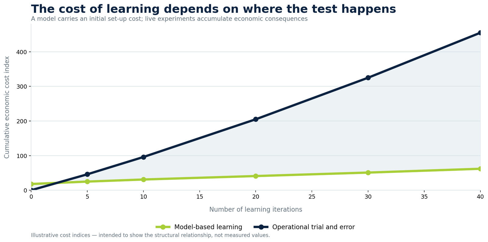
This advantage compounds:
Small and medium-sized businesses retain genuine advantages in speed, specialisation, proximity to customers, entrepreneurship and organisational flexibility. But flexibility is not permanently protected.
To remain cost-competitive, many businesses reduce employment and fixed professional capacity. Initially, this removes bureaucracy and waste. Beyond a certain point, further reduction removes the company’s ability to analyse, challenge, develop and renew itself.
The business becomes faster but progressively thinner.
It may remain legally independent while becoming economically dependent on a larger ecosystem for customer access, fulfilment, technology, payments, data and visibility. This is already familiar to merchants whose commercial viability depends on the rules and algorithms of major digital platforms.
A business can become operationally lean and strategically hollow at the same time.
Without accessible optimisation and learning infrastructure, many SMEs will face a narrowing set of structural routes: become a highly specialised microbusiness; join an ecosystem controlled by a larger platform; consolidate; surrender strategic functions to external providers; or exit the market.
This is a form of economic entropy. Data fragment, assumptions age, processes accumulate exceptions, technology decays and decision quality separates from operational reality. Preventing that deterioration requires continuous inputs of information, learning and renewal.
Optimisation is the work required to preserve coherence, value and independent capability.
Competition between learning systems
When two companies face the same repetitive decision environment, the company that can learn faster, test more alternatives and reduce the cost of error holds a structural advantage.
Competitiveness then ceases to be only a competition between ideas.
It becomes a competition between learning systems.
A brilliant initial idea can be surpassed by an organisation capable of testing, correcting and scaling a reasonable idea through hundreds of low-cost iterations.
The purpose of optimisation technology for SMEs is not to reproduce the entire analytical structure of a large corporation. It is to reduce the cost of each reliable iteration until evidence-based learning becomes operationally affordable.
That is the larger effort behind CF Compass and the wider optimisation mission: to help businesses test decisions before committing scarce resources, improve their models as new evidence arrives and preserve the analytical capacity required for independent renewal.
If optimisation remains affordable only at scale, market concentration is not an accidental outcome. It is the predictable result of unequal learning economics.
Evolution, not elimination
Optimisation is a game changer, not a bogeyman—and certainly not a corporate swear word. Properly designed optimisation models are not built to strip a business down until nothing remains. They help it learn, adapt, protect scarce capacity and evolve with less waste and fewer destructive mistakes. The purpose is evolution, not elimination.